1 Understanding Large Language Models
This chapter covers
- High-level explanations of the fundamental concepts behind large language models (LLMs)
- Insights into the transformer architecture from which ChatGPT-like LLMs are derived
- A plan for building an LLM from scratch
Large language models (LLMs) like ChatGPT are deep neural network models developed over the last few years. They ushered in a new era for Natural Language Processing (NLP). Before the advent of large language models, traditional methods excelled at categorization tasks such as email spam classification and straightforward pattern recognition that could be captured with handcrafted rules or simpler models. However, they typically underperformed in language tasks that demanded complex understanding and generation abilities, such as parsing detailed instructions, conducting contextual analysis, or creating coherent and contextually appropriate original text. For example, previous generations of language models could not write an email from a list of keywords—a task that is trivial for contemporary LLMs.
LLMs have remarkable capabilities to understand, generate, and interpret human language. However, it's important to clarify that when we say language models "understand," we mean that they can process and generate text in ways that appear coherent and contextually relevant, not that they possess human-like consciousness or comprehension.
Enabled by advancements in deep learning, which is a subset of machine learning and artificial intelligence (AI) focused on neural networks, LLMs are trained on vast quantities of text data. This allows LLMs to capture deeper contextual information and subtleties of human language compared to previous approaches. As a result, LLMs have significantly improved performance in a wide range of NLP tasks, including text translation, sentiment analysis, question answering, and many more.
Another important distinction between contemporary LLMs and earlier NLP models is that the latter were typically designed for specific tasks; whereas those earlier NLP models excelled in their narrow applications, LLMs demonstrate a broader proficiency across a wide range of NLP tasks.
The success behind LLMs can be attributed to the transformer architecture which underpins many LLMs, and the vast amounts of data LLMs are trained on, allowing them to capture a wide variety of linguistic nuances, contexts, and patterns that would be challenging to manually encode.
This shift towards implementing models based on the transformer architecture and using large training datasets to train LLMs has fundamentally transformed NLP, providing more capable tools for understanding and interacting with human language.
Beginning with this chapter, we set the foundation to accomplish the primary objective of this book: understanding LLMs by implementing a ChatGPT-like LLM based on the transformer architecture step by step in code.
1.1 What is an LLM?
An LLM, a large language model, is a neural network designed to understand, generate, and respond to human-like text. These models are deep neural networks trained on massive amounts of text data, sometimes encompassing large portions of the entire publicly available text on the internet.
The "large" in large language model refers to both the model's size in terms of parameters and the immense dataset on which it's trained. Models like this often have tens or even hundreds of billions of parameters, which are the adjustable weights in the network that are optimized during training to predict the next word in a sequence. Next-word prediction is sensible because it harnesses the inherent sequential nature of language to train models on understanding context, structure, and relationships within text. Yet, it is a very simple task and so it issurprising to many researchers that it can produce such capable models. We will discuss and implement the next-word training procedure in later chapters step by step.
LLMs utilize an architecture called the transformer (covered in more detail in section 1.4), which allows them to pay selective attention to different parts of the input when making predictions, making them especially adept at handling the nuances and complexities of human language.
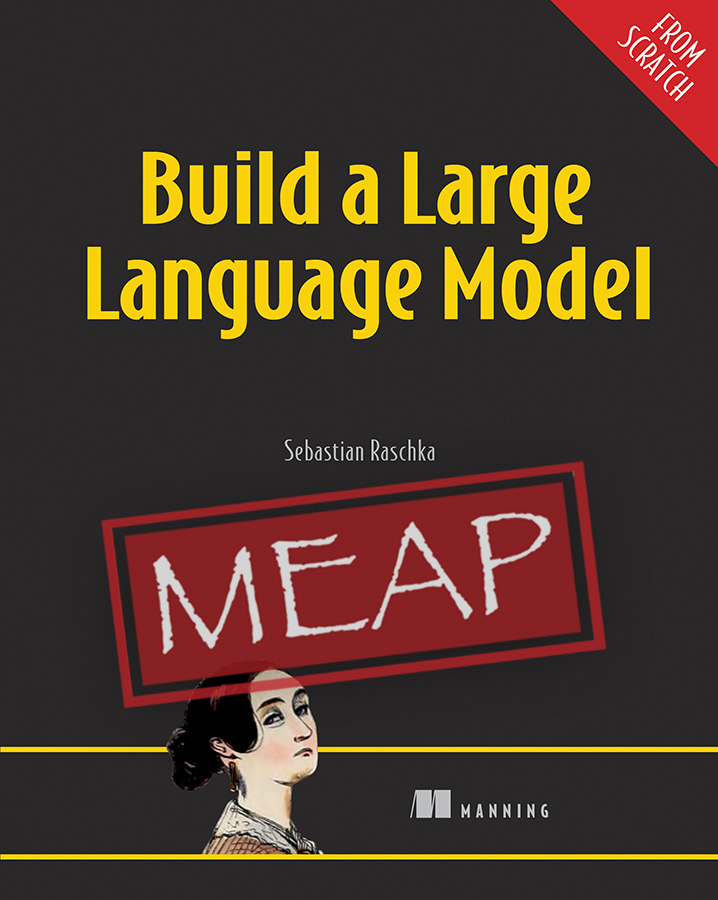
Since LLMs are capable of generating text, LLMs are also often referred to as a form of generative artificial intelligence (AI), often abbreviated as generative AI or GenAI. As illustrated in figure 1.1, AI encompasses the broader field of creating machines that can perform tasks requiring human-like intelligence, including understanding language, recognizing patterns, and making decisions, and includes subfields like machine learning and deep learning.
Figure 1.1 As this hierarchical depiction of the relationship between the different fields suggests, LLMs represent a specific application of deep learning techniques, leveraging their ability to process and generate human-like text. Deep learning is a specialized branch of machine learning that focuses on using multi-layer neural networks. And machine learning and deep learning are fields aimed at implementing algorithms that enable computers to learn from data and perform tasks that typically require human intelligence. The field of artificial intelligence is nowadays dominated by machine learning and deep learning but it also includes other approaches, for example by using rule-based systems, genetic algorithms, expert systems, fuzzy logic, or symbolic reasoning.
The algorithms used to implement AI are the focus of the field of machine learning. Specifically, machine learning involves the development of algorithms that can learn from and make predictions or decisions based on data without being explicitly programmed. To illustrate this, imagine a spam filter as a practical application of machine learning. Instead of manually writing rules to identify spam emails, a machine learning algorithm is fed examples of emails labeled as spam and legitimate emails. By minimizing theerror in its predictions on a training dataset, the model then learns to recognize patterns and characteristics indicative of spam, enabling it to classify new emails as either spam or legitimate.
Deep learning is a subset of machine learning that focuses on utilizing neural networks with three or more layers (also called deep neural networks) to model complex patterns and abstractions in data. In contrast to deep learning, traditional machine learning requires manual feature extraction. This means that human experts need to identify and select the most relevant features for the model.
Returning to the spam classification example, in traditional machine learning, human experts might manually extract features from email text such as the frequency of certain trigger words ("prize," "win," "free"), the number of exclamation marks, use of all uppercase words, or the presence of suspicious links. This dataset, created based on these expert-defined features, would then be used to train the model. In contrast to traditional machine learning, deep learning does not require manual feature extraction. This means that human experts do not need to identify and select the most relevant features for a deep learning model
The upcoming sections will cover some of the problems LLMs can solve today, the challenges that LLMs address, and the general LLM architecture, which we will implement in this book.
1.2 Applications of LLMs
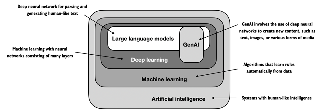
Owing to their advanced capabilities to parse and understand unstructured text data, LLMs have a broad range of applications across various domains. Today, LLMs are employed for machine translation, generation of novel texts (see figure 1.2), sentiment analysis, text summarization, and many other tasks. LLMs have recently been used for content creation, such as writing fiction, articles, and even computer code.
Figure 1.2 LLM interfaces enable natural language communication between users and AI systems. This screenshot shows ChatGPT writing a poem that according to a user's specifications.
LLMs can also power sophisticated chatbots and virtual assistants, such as OpenAI's ChatGPT or Google's Bard, which can answer user queries and augment traditional search engines such as Google Search or Microsoft Bing.
Moreover, LLMs may be used for effective knowledge retrieval from vast volumes of text in specialized areas such as medicine or law. This includes sifting through documents, summarizing lengthy passages, and answering technical questions.
In short, LLMs are invaluable for automating almost any task that involves parsing and generating text. Their applications are virtually endless, and as we continue to innovate and explore new ways to use these models, it's clear that LLMs have the potential to redefine our relationship with technology, making it more conversational, intuitive, and accessible.
In this book, we will focus on understanding how LLMs work from the ground up, coding an LLM that can generate texts. We will also learn about techniques that allow LLMs to carry out queries, ranging from answering questions to summarizing text, translating text into different languages, and more. In other words, in this book, we will learn how complex LLM assistants such as ChatGPT work by building one step by step.
1.3 Stages of building and using LLMs
Why should we build our own LLMs? Coding an LLM from the ground up is an excellent exercise to understand its mechanics and limitations. Also, it equips us with the required knowledge for pretaining or finetuning existing open-source LLM architectures to our own domain-specific datasets or tasks.
Research has shown that when it comes to modeling performance, custom-built LLMs—those tailored for specific tasks or domains—can outperform general-purpose LLMs like ChatGPT, which are designed for a wide array of applications. Examples of this include BloombergGPT, which is specialized for finance, and LLMs that are tailored for medical question answering (please see the Further Reading and References section at the end of this chapter for more details).
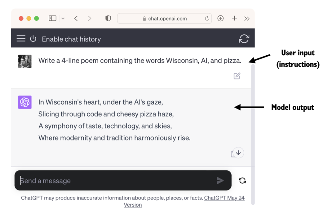
The general process of creating an LLM, including pretraining and finetuning. The term "pre" in "pretraining" refers to the initial phase where a model like an LLM is trained on a large, diverse dataset to develop a broad understanding of language. This pretrained model then serves as a foundational resource that can be further refined through finetuning, a process where the model is specifically trained on a narrower dataset that is more specific to particular tasks or domains. This two-stage training approach consisting of pretraining and finetuning is depicted in figure 1.3.
Figure 1.3 Pretraining an LLM involves next-word prediction on large unlabeled text corpora (raw text). A pretrained LLM can then be finetuned using a smaller labeled dataset.
As illustrated in figure 1.3, the first step in creating an LLM is to train it in on a large corpus of text data, sometimes referred to as raw text. Here, "raw" refers to the fact that this data is just regular text without any labeling information[1]. (Filtering may be applied, such as removing formatting characters or documents in unknown languages.)
This first training stage of an LLM is also known as pretraining, creating an initial pretrained LLM, often called a base or foundation model. A typical example of such a model is the GPT-3 model (the precursor of ChatGPT). This model is capable of text completion, that is, finishing a half-written sentence provided by a user. It also has limited few-shot capabilities, which means it can learn to perform new tasks based on only a few examples instead of needing extensive training data. This is further illustrated in the next section, Using transformers for different tasks.
After obtaining a pretrained LLM from training on unlabeled texts, we can further train the LLM on labeled data, also known as finetuning.
The two most popular categories of finetuning LLMs include instruction-finetuning and finetuning for classification tasks. In instruction-finetuning, the labeled dataset consists of instruction and answer pairs, such as a query to translate a text accompanied by the correctly translated text. In classification finetuning, the labeled dataset consists of texts and associated class labels, for example, emails associated with spam and non-spam labels.
In this book, we will cover both code implementations for pretraining and finetuning LLM, and we will delve deeper into the specifics of instruction-finetuning and finetuning for classification later in this book after pretraining a base LLM.
1.4 Using LLMs for different tasks
Most modern LLMs rely on the transformer architecture, which is a deep neural network architecture introduced in the 2017 paper Attention Is All You Need. To understand LLMs we briefly have to go over the original transformer, which was originally developed for machine translation, translating English texts to German and French. A simplified version of the transformer architecture is depicted in figure 1.4.
Figure 1.4 A simplified depiction of the original transformer architecture, which is a deep learning model for language translation. The transformer consists of two parts, an encoder that processes the input text and produces an embedding representation (a numerical representation that captures many different factors in different dimensions) of the text that the decoder can use to generate the translated text one word at a time. Note that this figure shows the final stage of the translation process where the decoder has to generate only the final word ("Beispiel"), given the original input text ("This is an example") and a partially translated sentence ("Das ist ein"), to complete the translation. The figure numbering indicates the sequence in which the data is processed and provides guidance on the optimal order to read the figure.
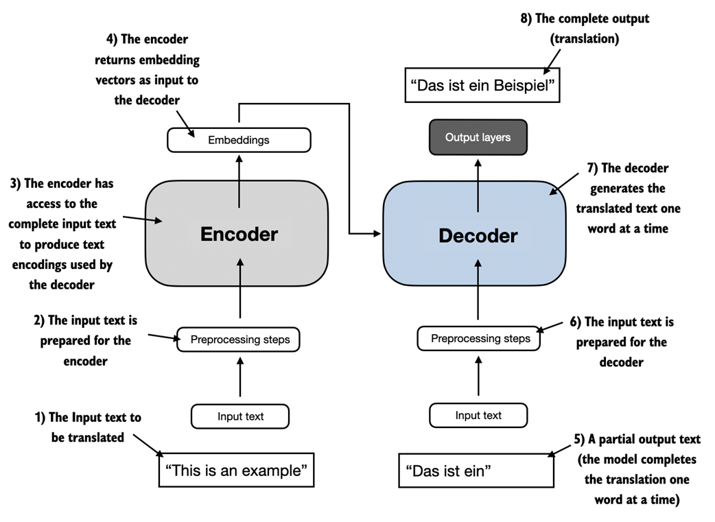
The transformer architecture depicted in figure 1.4 consists of two submodules, an encoder and a decoder. The encoder module processes the input text and encodes it into a series of numerical representations or vectors that capture the contextual information of the input. Then, the decoder module takes these encoded vectors and generates the output text from them. In a translation task, for example, the encoder would encode the text from the source language into vectors, and the decoder would decode these vectors to generate text in the target language.. Both the encoder and decoder consist of many layers connected by a so-called self-attention mechanism. You may have many questions regarding how the inputs are preprocessed and encoded. These will be addressed in a step-by-step implementation in the subsequent chapters.
A key component of transformers and LLMs is the self-attention mechanism (not shown), which allows the model to weigh the importance of different words or tokens in a sequence relative to each other. This mechanism enables the model to capture long-range dependencies and contextual relationships within the input data, enhancing its ability to generate coherent and contextually relevant output. However, due to its complexity, we will defer the explanation to Chapter 3, where we will discuss and implement it step by step. Moreover, we will also discuss and implement the data preprocessing steps to create the model inputs in Chapter 2, Working with Text Data.
Later variants of the transformer architecture, such as the so-called BERT (short for bidirectional encoder representations from transformers) and the various GPT models (short for generative pretrained transformers), built on this concept to adapt this architecture for different tasks. (References can be found in the Further Reading section at the end of this chapter.)
BERT, which is built upon the original transformer's encoder submodule, differs in its training approach from GPT. While GPT is designed for generative tasks, BERT and its variants specialize in masked word prediction, where the model predicts masked or hidden words in a given sentence as illustrated in figure 1.5. This unique training strategy equips BERT with strengths in text classification tasks, including sentiment prediction and document categorization. As an application of its capabilities, as of this writing, Twitter uses BERT to detect toxic content.
Figure 1.5 A visual representation of the transformer's encoder and decoder submodules. On the left, the encoder segment exemplifies BERT-like LLMs, which focus on masked word prediction and are primarily used for tasks like text classification. On the right, the decoder segment showcases GPT-like LLMs, designed for generative tasks and producing coherent text sequences.
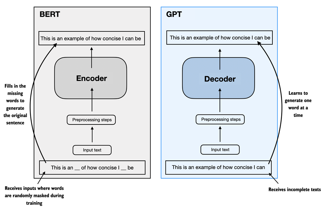
GPT, on the other hand, focuses on the decoder portion of the original transformer architecture and is designed for tasks that require generating texts. This includes machine translation, text summarization, fiction writing, writing computer code, and more. We will discuss the GPT architecture in more detail in the remaining sections of this chapter and implement it from scratch in this book.
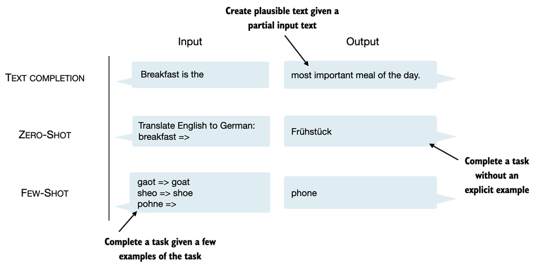
GPT models, primarily designed and trained to perform text completion tasks, also show remarkable versatility in their capabilities. These models are adept at executing both zero-shot and few-shot learning tasks. Zero-shot learning refers to the ability to generalize to completely unseen tasks without any prior specific examples. On the other hand, few-shot learning involves learning from a minimal number of examples the user provides as input, as shown in figure 1.6.
Figure 1.6 Next to text completion, GPT-like LLMs can solve various tasks based on their inputs without needing retraining, finetuning, or task-specific model architecture changes. Sometimes, it is helpful to provide examples of the target within the input, which is known as a few-shot setting. However, GPT-like LLMs are also capable of carrying out tasks without a specific example, which is called zero-shot setting.
Transformers versus LLMs
Today's LLMs are based on the transformer architecture introduced in the previous section. Hence, transformers and LLMs are terms that are often used synonymously in the literature. However, note that not all transformers are LLMs since transformers can also be used for computer vision. Also, not all LLMs are transformers, as there are large language models based on recurrent and convolutional architectures. The main motivation behind these alternative approaches is to improve the computational efficiency of LLMs. However, whether these alternative LLM architectures can compete with the capabilities of transformer-based LLMs and whether they are going to be adopted in practice remains to be seen. (Interested readers can find literature references describing these architectures in the Further Reading section at the end of this chapter.)
1.5 Utilizing large datasets
The large training datasets for popular GPT- and BERT-like models represent diverse and comprehensive text corpora encompassing billions of words, which include a vast array of topics and natural and computer languages. To provide a concrete example, table 1.1 summarizes the dataset used for pretraining GPT-3, which served as the base model for the first version of ChatGPT.
Table 1.1 The pretraining dataset of the popular GPT-3 LLM
| Dataset name | Dataset description | Number of tokens | Proportion in training data |
| CommonCrawl (filtered) | Web crawl data | 410 billion | 60% |
| WebText2 | Web crawl data | 19 billion | 22% |
| Books1 | Internet-based book corpus | 12 billion | 8% |
| Books2 | Internet-based book corpus | 55 billion | 8% |
| Wikipedia | High-quality text | 3 billion | 3% |
Table 1.1 reports the number of tokens, where a token is a unit of text that a model reads, and the number of tokens in a dataset is roughly equivalent to the number of words and punctuation characters in the text. We will cover tokenization, the process of converting text into tokens, in more detail in the next chapter.
The main takeaway is that the scale and diversity of this training dataset allows these models to perform well on diverse tasks including language syntax, semantics, and context, and even some requiring general knowledge.
GPT-3 dataset details
Note that each subset in table 1.1 was sampled 300 billion tokens, which implies that not all datasets were seen completely, and some were seen multiple times. The proportion column, ignoring rounding, adds to 100%. For reference, the 410 billion tokens in the CommonCrawl dataset require approximately 570 GB of storage. Later models based on GPT-3, for example, Meta's LLaMA, also include research papers from Arxiv (92 GB) and code-related Q&As from StackExchange (78 GB).
The Wikipedia corpus consists of English-language Wikipedia. While the authors of the GPT-3 paper didn't further specify the details, Books1 is likely a sample from Project Gutenberg (https://www.gutenberg.org/), and Books2 is likely from Libgen (https://en.wikipedia.org/wiki/Library_Genesis). CommonCrawl is a filtered subset of the CommonCrawl database (https://commoncrawl.org/), and WebText2 is the text of web pages from all outbound Reddit links from posts with 3+ upvotes.
The authors of the GPT-3 paper did not share the training dataset but a comparable dataset that is publicly available is The Pile (https://pile.eleuther.ai/). However, the collection may contain copyrighted works, and the exact usage terms may depend on the intended use case and country. For more information, see the HackerNews discussion at https://news.ycombinator.com/item?id=25607809.
The pretrained nature of these models makes them incredibly versatile for further finetuning on downstream tasks, which is why they are also known as base or foundation models. Pretraining LLMs requires access to significant resources and is very expensive. For example, the GPT-3 pretraining cost is estimated to be $4.6 million in terms of cloud computing credits[2].
The good news is that many pretrained LLMs, available as open-source models, can be used as general purpose tools to write, extract, and edit texts that were not part of the training data. Also, LLMs can be finetuned on specific tasks with relatively smaller datasets, reducing the computational resources needed and improving performance on the specific task.
In this book, we will implement the code for pretraining and use it to pretrain an LLM for educational purposes.. All computations will be executable on consumer hardware. After implementing the pretraining code we will learn how to reuse openly available model weights and load them into the architecture we will implement, allowing us to skip the expensive pretraining stage when we finetune LLMs later in this book.
1.6 A closer look at the GPT architecture
Previously in this chapter, we mentioned the terms GPT-like models, GPT-3, and ChatGPT. Let's now take a closer look at the general GPT architecture. First, GPT stands for Generative Pretrained Transformer and was originally introduced in the following paper:
- Improving Language Understanding by Generative Pre-Training (2018) by Radford et al. from OpenAI, http://cdn.openai.com/research-covers/language-unsupervised/language_understanding_paper.pdf
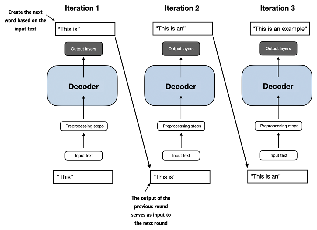
GPT-3 is a scaled-up version of this model that has more parameters and was trained on a larger dataset. And the original ChatGPT model was created by finetuning GPT-3 on a large instruction dataset using a method from OpenAI'sInstructGPT paper, which we will cover in more detail in Chapter 8, Finetuning with Human Feedback To Follow Instructions. As we have seen earlier in figure 1.6, these models are competent text completion models and can carry out other tasks such as spelling correction, classification, or language translation. This is actually very remarkable given that GPT models are pretrained on a relatively simple next-word prediction task, as illustrated in figure 1.7.
Figure 1.7 In the next-word pretraining task for GPT models, the system learns to predict the upcoming word in a sentence by looking at the words that have come before it. This approach helps the model understand how words and phrases typically fit together in language, forming a foundation that can be applied to various other tasks.
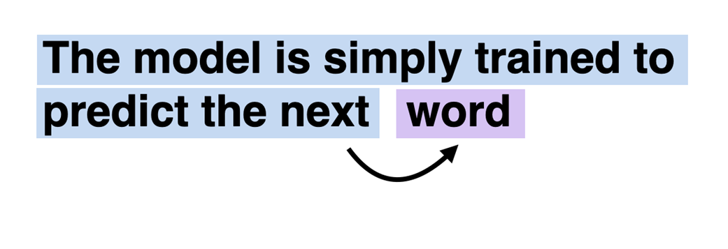
The next-word prediction task is a form of self-supervised learning, which is a form of self-labeling. This means that we don't need to collect labels for the training data explicitly but can leverage the structure of the data itself: we can use the next word in a sentence or document as the label that the model is supposed to predict. Since this next-word prediction task allows us to create labels "on the fly," it is possible to leverage massive unlabeled text datasets to train LLMs as previously discussed in section 1.5, Utilizing large datasets.
Compared to the original transformer architecture we covered in section 1.4, Using LLMs for different tasks, the general GPT architecture is relatively simple. Essentially, it's just the decoder part without the encoder as illustrated in figure 1.8. Since decoder-style models like GPT generate text by predicting text one word at a time, they are considered a type of autoregressive model.
Architectures such as GPT-3 are also significantly larger than the original transformer model. For instance, the original transformer repeated the encoder and decoder blocks six times. GPT-3 has 96 transformer layers and 175 billion parameters in total.
Figure 1.8 The GPT architecture, employs only the decoder portion of the original transformer. It is designed for unidirectional, left-to-right processing, making it well-suited for text generation and next-word prediction tasks to generate text in iterative fashion one word at a time.
GPT-3 was introduced in 2020, which is a long time ago by the standard of deep learning and LLM development, more recent architectures like Meta's Llama models are still based on the same underlying concepts, introducing only minor modifications. Hence, understanding GPT remains as relevant as ever, and this book focuses on implementing the prominent architecture behind GPT while providing pointers to specific tweaks employed by alternative LLMs.
Lastly, it's interesting to note that although the original transformer model was explicitly designed for language translation, GPT models—despite their larger yet simpler architecture aimed at next-word prediction—are also capable of performing translation tasks. This capability was initially unexpected to researchers, as it emerged from a model primarily trained on a next-word prediction task, which is a task that did not specifically target translation.
The ability to perform tasks that the model wasn't explicitly trained to perform is called an "emerging property." This capability isn't explicitly taught during training but emerges as a natural consequence of the model's exposure to vast quantities of multilingual data in diverse contexts. The fact that GPT models can "learn" the translation patterns between languages and perform translation tasks even though they weren't specifically trained for it demonstrates the benefits and capabilities of these large-scale, generative language models. We can perform diverse tasks without using diverse models for each.
1.7 Building a large language model
In this chapter, we laid the groundwork for understanding LLMs. In the remainder of this book, we will be coding one from scratch. We will take the fundamental idea behind GPT as a blueprint and tackle this in three stages, as outlined in figure 1.9.
Figure 1.9 The stages of building LLMs covered in this book include implementing the LLM architecture and data preparation process, pretraining an LLM to create a foundation model, and finetuning the foundation model to become a personal assistant or text classifier.
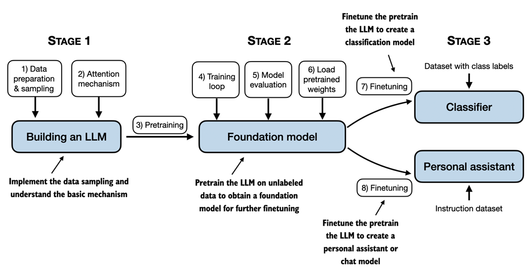
First, we will learn about the fundamental data preprocessing steps and code the attention mechanism that is at the heart of every LLM.
Next, in stage 2, we will learn how to code and pretrain a GPT-like LLM capable of generating new texts. And we will also go over the fundamentals of evaluating LLMs, which is essential for developing capable NLP systems.
Note that pretraining a large LLM from scratch is a significant endeavor, demanding thousands to millions of dollars in computing costs for GPT-like models. Therefore, the focus of stage 2 is on implementing training for educational purposes using a small dataset. In addition, the book will also provide code examples for loading openly available model weights.
Finally, in stage 3, we will take a pretrained LLM and finetune it to follow instructions such as answering queries or classifying texts -- the most common tasks in many real-world applications and research.
I hope you are looking forward to embarking on this exciting journey!
1.8 Summary
- LLMs have transformed the field of natural language processing, which previouslyrelied on explicit rule-based systems and simpler statistical methods. The advent of LLMs introduced new deep learning-driven approaches that led to advancements in understanding, generating, and translating human language.
- Modern LLMs are trained in two main steps.
- First, they are pretrained on a large corpus of unlabeled text by using the prediction of the next word in a sentence as a "label."
- Then, they are finetuned on a smaller, labeled target dataset to follow instructions or perform classification tasks.
- LLMs are based on the transformer architecture. The key idea of the transformer architecture is an attention mechanism that gives the LLM selective access to the whole input sequence when generating the output one word at a time.
- The original transformer architecture consists of an encoder for parsing text and a decoder for generating text.
- LLMs for generating text and following instructions, such as GPT-3 and ChatGPT, only implement decoder modules, simplifying the architecture.
- Large datasets consisting of billions of words are essential for pretraining LLMs. in this book, we will implement and train LLMs on small datasets for educational purposes but also see how we can load openly available model weights.
- While the general pretraining task for GPT-like models is to predict the next word in a sentence, these LLMs exhibit "emergent" properties such as capabilities to classify, translate, or summarize texts.
- Once an LLM is pretrained, the resulting foundation model can be finetuned more efficiently for various downstream tasks.
- LLMs finetuned on custom datasets can outperform general LLMs on specific tasks.
1.9 References and further reading
Custom-built LLMs are able to outperform general-purpose LLMs as a team at Bloomberg showed via a a version of GPT pretrained on finance data from scratch. The custom LLM outperformed ChatGPT on financial tasks while maintaining good performance on general LLM benchmarks:
- BloombergGPT: A Large Language Model for Finance (2023) by Wu et al., https://arxiv.org/abs/2303.17564
- Existing LLMs can be adapted and finetuned to outperform general LLMs as well, which teams from Google Research and Google DeepMind showed in a medical context:
- Towards Expert-Level Medical Question Answering with Large Language Models (2023) by Singhal et al., https://arxiv.org/abs/2305.09617
- The paper that proposed the original transformer architecture:
- Attention Is All You Need (2017) by Vaswani et al., https://arxiv.org/abs/1706.03762
- The original encoder-style transformer, called BERT:
- BERT: Pre-training of Deep Bidirectional Transformers for Language Understanding (2018) by Devlin et al., https://arxiv.org/abs/1810.04805.
- The paper describing the decoder-style GPT-3 model, which inspired modern LLMs and will be used as a template for implementing an LLM from scratch in this book:
- Language Models are Few-Shot Learners (2020) by Brown et al., https://arxiv.org/abs/2005.14165.
- The original vision transformer for classifying images, which illustrates that transformer architectures are not only restricted to text inputs:
- An Image is Worth 16x16 Words: Transformers for Image Recognition at Scale (2020) by Dosovitskiy et al., https://arxiv.org/abs/2010.11929
- Two experimental (but less popular) LLM architectures that serve as examples that not all LLMs need to be based on the transformer architecture:
- RWKV: Reinventing RNNs for the Transformer Era (2023) by Peng et al., https://arxiv.org/abs/2305.13048
- Hyena Hierarchy: Towards Larger Convolutional Language Models (2023) by Poli et al., https://arxiv.org/abs/2302.10866
- Meta AI's model is a popular implementation of a GPT-like model that is openly available in contrast to GPT-3 and ChatGPT:
- Llama 2: Open Foundation and Fine-Tuned Chat Models (2023) by Touvron et al., https://arxiv.org/abs/2307.092881
- For readers interested in additional details about the dataset references in section 1.5, this paper describes the publicly available The Pile dataset curated by Eleuther AI:
- The Pile: An 800GB Dataset of Diverse Text for Language Modeling (2020) by Gao et al., https://arxiv.org/abs/2101.00027.
- Training Language Models to Follow Instructions with Human Feedback (2022) by Ouyang et al., https://arxiv.org/abs/2203.02155
[1] Readers with a background in machine learning may note that labeling information is typically required for traditional machine learning models and deep neural networks trained via the conventional supervised learning paradigm. However, this is not the case for the pretraining stage of LLMs. In this phase, LLMs leverage self-supervised learning, where the model generates its own labels from the input data. This concept is covered later in this chapter
[2] GPT-3, The $4,600,000 Language Model, https://www.reddit.com/r/MachineLearning/comments/h0jwoz/d_gpt3_the_4600000_language_model/
2 Working with Text Data
This chapter covers
- Preparing text for large language model training
- Splitting text into word and subword tokens
- Byte pair encoding as a more advanced way of tokenizing text
- Sampling training examples with a sliding window approach
- Converting tokens into vectors that feed into a large language model
In the previous chapter, we delved into the general structure of large language models (LLMs) and learned that they are pretrained on vast amounts of text. Specifically, our focus was on decoder-only LLMs based on the transformer architecture, which underlies ChatGPT and other popular GPT-like LLMs.
During the pretraining stage, LLMs process text one word at a time. Training LLMs with millions to billions of parameters using a next-word prediction task yields models with impressive capabilities. These models can then be further finetuned to follow general instructions or perform specific target tasks. But before we can implement and train LLMs in the upcoming chapters, we need to prepare the training dataset, which is the focus of this chapter, as illustrated in figure 2.1
Figure 2.1 A mental model of the three main stages of coding an LLM, pretraining the LLM on a general text dataset, and finetuning it on a labeled dataset. This chapter will explain and code the data preparation and sampling pipeline that provides the LLM with the text data for pretraining.
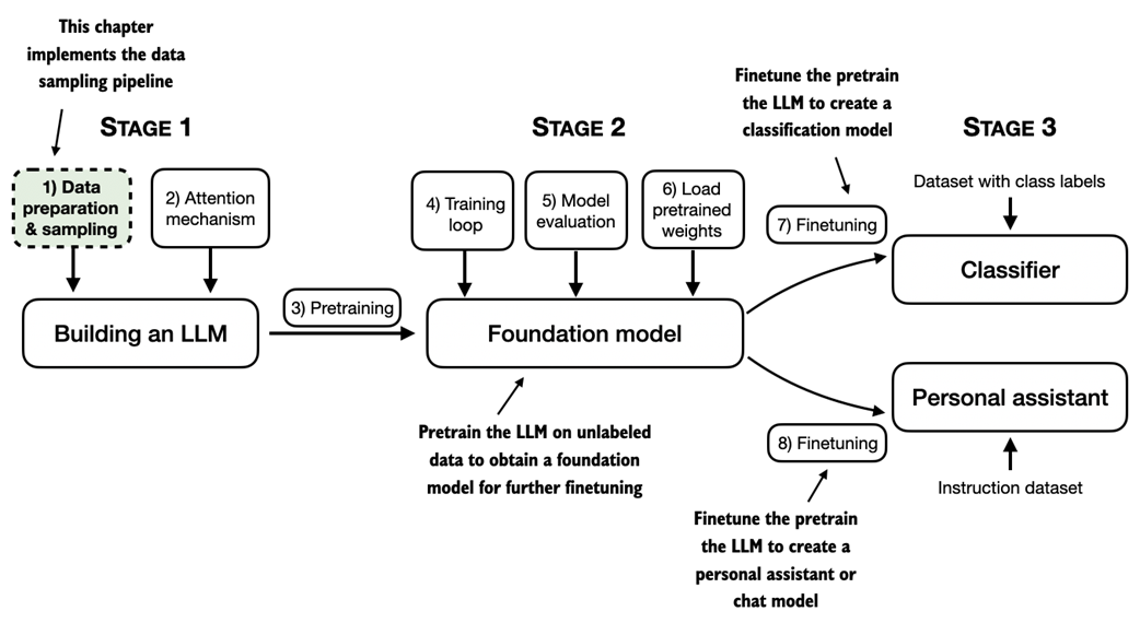
In this chapter, you'll learn how to prepare input text for training LLMs. This involves splitting text into individual word and subword tokens, which can then be encoded into vector representations for the LLM. You'll also learn about advanced tokenization schemes like byte pair encoding, which is utilized in popular LLMs like GPT. Lastly, we'll implement a sampling and data loading strategy to produce the input-output pairs necessary for training LLMs in subsequent chapters.
2.1 Understanding word embeddings
Deep neural network models, including LLMs, cannot process raw text directly. Since text is categorical, it isn't compatible with the mathematical operations used to implement and train neural networks. Therefore, we need a way to represent words as continuous-valued vectors. (Readers unfamiliar with vectors and tensors in a computational context can learn more in Appendix A, section A2.2 Understanding tensors.)
The concept of converting data into a vector format is often referred to as embedding. Using a specific neural network layer or another pretrained neural network model, we can embed different data types, for example, video, audio, and text, as illustrated in figure 2.2.
Figure 2.2 Deep learning models cannot process data formats like video, audio, and text in their raw form. Thus, we use an embedding model to transform this raw data into a dense vector representation that deep learning architectures can easily understand and process. Specifically, this figure illustrates the process of converting raw data into a three-dimensional numerical vector. It's important to note that different data formats require distinct embedding models. For example, an embedding model designed for text would not be suitable for embedding audio or video data.
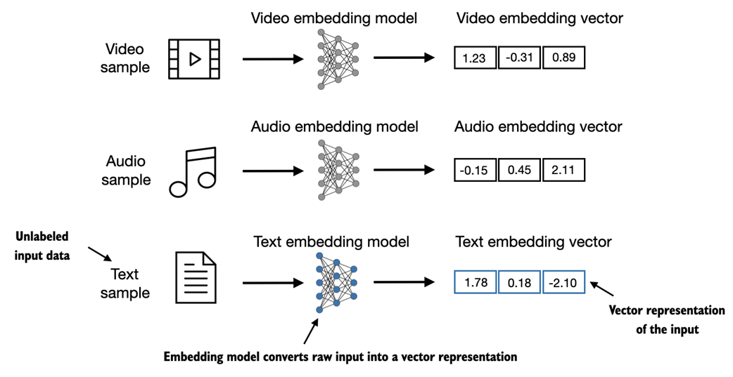
At its core, an embedding is a mapping from discrete objects, such as words, images, or even entire documents, to points in a continuous vector space -- the primary purpose of embeddings is to convert non-numeric data into a format that neural networks can process.
While word embeddings are the most common form of text embedding, there are also embeddings for sentences, paragraphs, or whole documents. Sentence or paragraph embeddings are popular choices for retrieval-augmented generation. Retrieval-augmented generation combines generation (like producing text) with retrieval (like searching an external knowledge base) to pull relevant information when generating text, which is a technique that is beyond the scope of this book. Since our goal is to train GPT-like LLMs, which learn to generate text one word at a time, this chapter focuses on word embeddings.
There are several algorithms and frameworks that have been developed to generate word embeddings. One of the earlier and most popular examples is the Word2Vec approach. Word2Vec trained neural network architecture to generate word embeddings by predicting the context of a word given the target word or vice versa. The main idea behind Word2Vec is that words that appear in similar contexts tend to have similar meanings. Consequently, when projected into 2-dimensional word embeddings for visualization purposes, it can be seen that similar terms cluster together, as shown in figure 2.3.
Figure 2.3 If word embeddings are two-dimensional, we can plot them in a two-dimensional scatterplot for visualization purposes as shown here. When using word embedding techniques, such as Word2Vec, words corresponding to similar concepts often appear close to each other in the embedding space. For instance, different types of birds appear closer to each other in the embedding space compared to countries and cities.
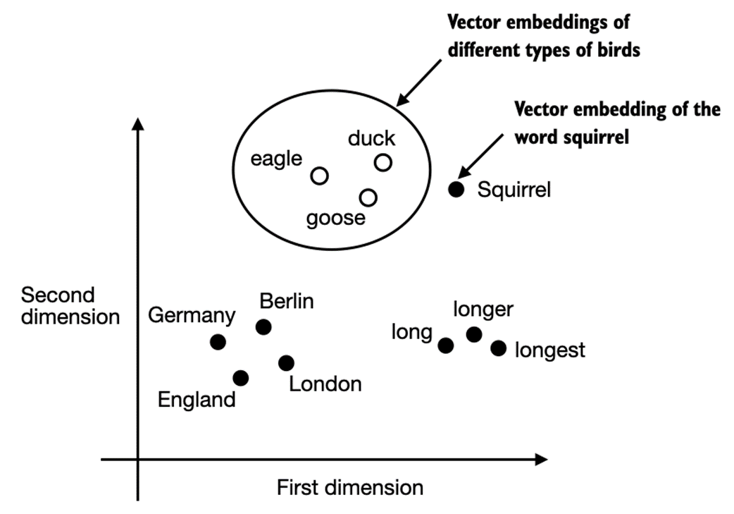
Word embeddings can have varying dimensions, from one to thousands. As shown in figure 2.3, we can choose two-dimensional word embeddings for visualization purposes. A higher dimensionality might capture more nuanced relationships but at the cost of computational efficiency.
While we can use pretrained models such as Word2Vec to generate embeddings for machine learning models, LLMs commonly produce their own embeddings that are part of the input layer and are updated during training. The advantage of optimizing the embeddings as part of the LLM training instead of using Word2Vec is that the embeddings are optimized to the specific task and data at hand. We will implement such embedding layers later in this chapter. Furthermore, LLMs can also create contextualized output embeddings, as we discuss in chapter 3.
Unfortunately, high-dimensional embeddings present a challenge for visualization because our sensory perception and common graphical representations are inherently limited to three dimensions or fewer, which is why figure 2.3 showed two-dimensional embeddings in a two-dimensional scatterplot. However, when working with LLMs, we typically use embeddings with a much higher dimensionality than shown in figure 2.3. For both GPT-2 and GPT-3, the embedding size (often referred to as the dimensionality of the model's hidden states) varies based on the specific model variant and size. It is a trade-off between performance and efficiency. The smallest GPT-2 (117M parameters) and GPT-3 (125 M parameters) models use an embedding size of 768 dimensions to provide concrete examples. The largest GPT-3 model (175B parameters) uses an embedding size of 12,288 dimensions.
The upcoming sections in this chapter will walk through the required steps for preparing the embeddings used by an LLM, which include splitting text into words, converting words into tokens, and turning tokens into embedding vectors.
2.2 Tokenizing text
This section covers how we split input text into individual tokens, a required preprocessing step for creating embeddings for an LLM. These tokens are either individual words or special characters, including punctuation characters, as shown in figure 2.4.
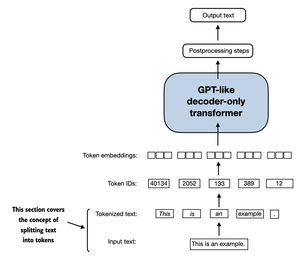
Figure 2.4 A view of the text processing steps covered in this section in the context of an LLM. Here, we split an input text into individual tokens, which are either words or special characters, such as punctuation characters. In upcoming sections, we will convert the text into token IDs and create token embeddings.
The text we will tokenize for LLM training is a short story by Edith Wharton called The Verdict, which has been released into the public domain and is thus permitted to be used for LLM training tasks. The text is available on Wikisource at https://en.wikisource.org/wiki/The_Verdict, and you can copy and paste it into a text file, which I copied into a text file "the-verdict.txt" to load using Python's standard file reading utilities:
Listing 2.1 Reading in a short story as text sample into Python
with open("the-verdict.txt", "r", encoding="utf-8") as f: raw_text = f.read() print("Total number of character:", len(raw_text)) print(raw_text[:99]) Alternatively, you can find this "the-verdict.txt" file in this book's GitHub repository at https://github.com/rasbt/LLMs-from-scratch/tree/main/ch02/01_main-chapter-code.
The print command prints the total number of characters followed by the first 100 characters of this file for illustration purposes:
Total number of character: 20479 I HAD always thought Jack Gisburn rather a cheap genius--though a good fellow enough--so it was no
Our goal is to tokenize this 20,479-character short story into individual words and special characters that we can then turn into embeddings for LLM training in the upcoming chapters.
Text sample sizes
Note that it's common to process millions of articles and hundreds of thousands of books -- many gigabytes of text -- when working with LLMs. However, for educational purposes, it's sufficient to work with smaller text samples like a single book to illustrate the main ideas behind the text processing steps and to make it possible to run it in reasonable time on consumer hardware.
How can we best split this text to obtain a list of tokens? For this, we go on a small excursion and use Python's regular expression library re for illustration purposes. (Note that you don't have to learn or memorize any regular expression syntax since we will transition to a pre-built tokenizer later in this chapter.)
Using some simple example text, we can use the re.split command with the following syntax to split a text on whitespace characters:
import re text = "Hello, world. This, is a test." result = re.split(r'(\s)', text) print(result)
The result is a list of individual words, whitespaces, and punctuation characters:
['Hello,', ' ', 'world.', ' ', 'This,', ' ', 'is', ' ', 'a', ' ', 'test.']
Note that the simple tokenization scheme above mostly works for separating the example text into individual words, however, some words are still connected to punctuation characters that we want to have as separate list entries.
Let's modify the regular expression splits on whitespaces (\s) and commas, and periods ([,.]):
result = re.split(r'([,.]|\s)', text) print(result)
We can see that the words and punctuation characters are now separate list entries just as we wanted:
['Hello', ',', '', ' ', 'world.', ' ', 'This', ',', '', ' ', 'is', ' ', 'a', ' ', 'test.']
A small remaining issue is that the list still includes whitespace characters. Optionally, we can remove these redundant characters safely remove as follows:
result = [item.strip() for item in result if item.strip()] print(result)
The resulting whitespace-free output looks like as follows:
['Hello', ',', 'world.', 'This', ',', 'is', 'a', 'test.']
Removing whitespaces or not
When developing a simple tokenizer, whether we should encode whitespaces as separate characters or just remove them depends on our application and its requirements. Removing whitespaces reduces the memory and computing requirements. However, keeping whitespaces can be useful if we train models that are sensitive to the exact structure of the text (for example, Python code, which is sensitive to indentation and spacing). Here, we remove whitespaces for simplicity and brevity of the tokenized outputs. Later, we will switch to a tokenization scheme that includes whitespaces.
The tokenization scheme we devised above works well on the simple sample text. Let's modify it a bit further so that it can also handle other types of punctuation, such as question marks, quotation marks, and the double-dashes we have seen earlier in the first 100 characters of Edith Wharton's short story, along with additional special characters:
text = "Hello, world. Is this-- a test?" result = re.split(r'([,.?_!"()\']|--|\s)', text) result = [item.strip() for item in result if item.strip()] print(result)
The resulting output is as follows:
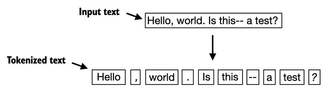
['Hello', ',', 'world', '.', 'Is', 'this', '--', 'a', 'test', '?']
As we can see based on the results summarized in figure 2.5, our tokenization scheme can now handle the various special characters in the text successfully.
Figure 2.5 The tokenization scheme we implemented so far splits text into individual words and punctuation characters. In the specific example shown in this figure, the sample text gets split into 10 individual tokens.
Now that we got a basic tokenizer working, let's apply it to Edith Wharton's entire short story:
preprocessed = re.split(r'([,.?_!"()\']|--|\s)', raw_text) preprocessed = [item.strip() for item in preprocessed if item.strip()] print(len(preprocessed))
The above print statement outputs 4649, which is the number of tokens in this text (without whitespaces).
Let's print the first 30 tokens for a quick visual check:
print(preprocessed[:30])
The resulting output shows that our tokenizer appears to be handling the text well since all words and special characters are neatly separated:
['I', 'HAD', 'always', 'thought', 'Jack', 'Gisburn', 'rather', 'a', 'cheap', 'genius', '--', 'though', 'a', 'good', 'fellow', 'enough', '--', 'so', 'it', 'was', 'no', 'great', 'surprise', 'to', 'me', 'to', 'hear', 'that', ',', 'in']
2.3 Converting tokens into token IDs
In the previous section, we tokenized a short story by Edith Wharton into individual tokens. In this section, we will convert these tokens from a Python string to an integer representation to produce the so-called token IDs. This conversion is an intermediate step before converting the token IDs into embedding vectors.
To map the previously generated tokens into token IDs, we have to build a so-called vocabulary first. This vocabulary defines how we map each unique word and special character to a unique integer, as shown in figure 2.6.
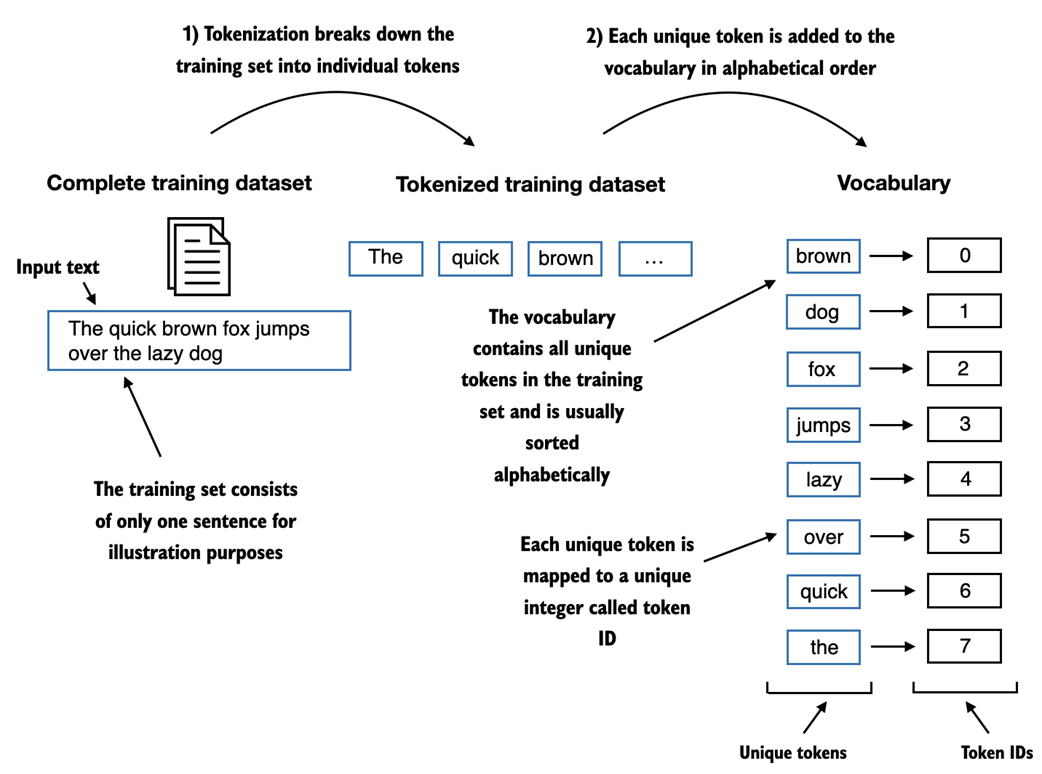
Figure 2.6 We build a vocabulary by tokenizing the entire text in a training dataset into individual tokens. These individual tokens are then sorted alphabetically, and unique tokens are removed. The unique tokens are then aggregated into a vocabulary that defines a mapping from each unique token to a unique integer value. The depicted vocabulary is purposefully small for illustration purposes and contains no punctuation or special characters for simplicity.
In the previous section, we tokenized Edith Wharton's short story and assigned it to a Python variable called preprocessed. Let's now create a list of all unique tokens and sort them alphabetically to determine the vocabulary size:
all_words = sorted(list(set(preprocessed))) vocab_size = len(all_words) print(vocab_size)
After determining that the vocabulary size is 1,159 via the above code, we create the vocabulary and print its first 50 entries for illustration purposes:
Listing 2.2 Creating a vocabulary
vocab = {token:integer for integer,token in enumerate(all_words)} for i, item in enumerate(vocab.items()): print(item) if i > 50: break The output is as follows:
('!', 0) ('"', 1) ("'", 2) ... ('Has', 49) ('He', 50) As we can see, based on the output above, the dictionary contains individual tokens associated with unique integer labels. Our next goal is to apply this vocabulary to convert new text into token IDs, as illustrated in figure 2.7.
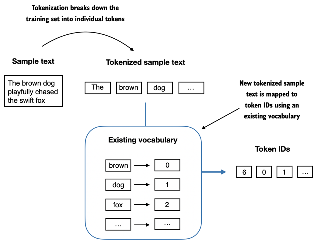
Figure 2.7 Starting with a new text sample, we tokenize the text and use the vocabulary to convert the text tokens into token IDs. The vocabulary is built from the entire training set and can be applied to the training set itself and any new text samples. The depicted vocabulary contains no punctuation or special characters for simplicity.
Later in this book, when we want to convert the outputs of an LLM from numbers back into text, we also need a way to turn token IDs into text. For this, we can create an inverse version of the vocabulary that maps token IDs back to corresponding text tokens.
Let's implement a complete tokenizer class in Python with an encode method that splits text into tokens and carries out the string-to-integer mapping to produce token IDs via the vocabulary. In addition, we implement a decode method that carries out the reverse integer-to-string mapping to convert the token IDs back into text.
The code for this tokenizer implementation is as in listing 2.3:
Listing 2.3 Implementing a simple text tokenizer
class SimpleTokenizerV1: def __init__(self, vocab): self.str_to_int = vocab #A self.int_to_str = {i:s for s,i in vocab.items()} #B def encode(self, text): #C preprocessed = re.split(r'([,.?_!"()\']|--|\s)', text) preprocessed = [item.strip() for item in preprocessed if item.strip()] ids = [self.str_to_int[s] for s in preprocessed] return ids def decode(self, ids): #D text = " ".join([self.int_to_str[i] for i in ids]) text = re.sub(r'\s+([,.?!"()\'])', r'\1', text) #E return text Using the SimpleTokenizerV1 Python class above, we can now instantiate new tokenizer objects via an existing vocabulary, which we can then use to encode and decode text, as illustrated in figure 2.8.
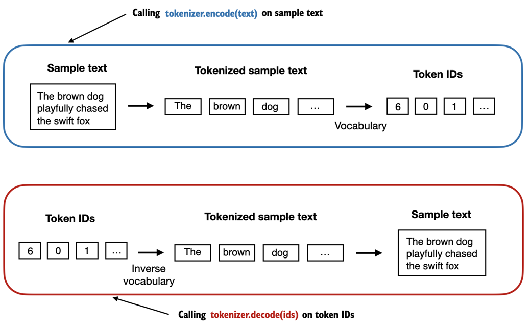
Figure 2.8 Tokenizer implementations share two common methods: an encode method and a decode method. The encode method takes in the sample text, splits it into individual tokens, and converts the tokens into token IDs via the vocabulary. The decode method takes in token IDs, converts them back into text tokens, and concatenates the text tokens into natural text.
Let's instantiate a new tokenizer object from the SimpleTokenizerV1 class and tokenize a passage from Edith Wharton's short story to try it out in practice:
tokenizer = SimpleTokenizerV1(vocab) text = """"It's the last he painted, you know," Mrs. Gisburn said with pardonable pride.""" ids = tokenizer.encode(text) print(ids)
The code above prints the following token IDs:
[1, 58, 2, 872, 1013, 615, 541, 763, 5, 1155, 608, 5, 1, 69, 7, 39, 873, 1136, 773, 812, 7]
Next, let's see if we can turn these token IDs back into text using the decode method:
tokenizer.decode(ids)
This outputs the following text:
'" It\' s the last he painted, you know," Mrs. Gisburn said with pardonable pride.'
Based on the output above, we can see that the decode method successfully converted the token IDs back into the original text.
So far, so good. We implemented a tokenizer capable of tokenizing and de-tokenizing text based on a snippet from the training set. Let's now apply it to a new text sample that is not contained in the training set:
text = "Hello, do you like tea?" tokenizer.encode(text)
Executing the code above will result in the following error:
... KeyError: 'Hello'
The problem is that the word "Hello" was not used in the The Verdict short story. Hence, it is not contained in the vocabulary. This highlights the need to consider large and diverse training sets to extend the vocabulary when working on LLMs.
In the next section, we will test the tokenizer further on text that contains unknown words, and we will also discuss additional special tokens that can be used to provide further context for an LLM during training.
2.4 Adding special context tokens
In the previous section, we implemented a simple tokenizer and applied it to a passage from the training set. In this section, we will modify this tokenizer to handle unknown words.
We will also discuss the usage and addition of special context tokens that can enhance a model's understanding of context or other relevant information in the text. These special tokens can include markers for unknown words and document boundaries, for example.
In particular, we will modify the vocabulary and tokenizer we implemented in the previous section, SimpleTokenizerV2, to support two new tokens, <|unk|> and <|endoftext|>, as illustrated in figure 2.8.
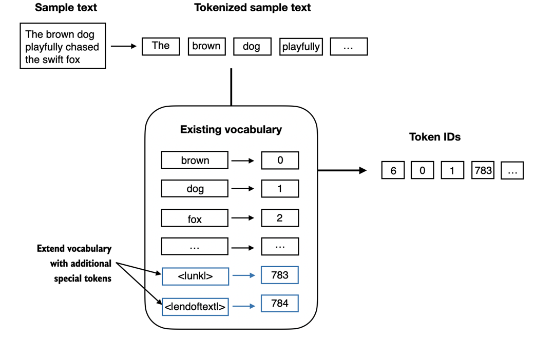
Figure 2.9 We add special tokens to a vocabulary to deal with certain contexts. For instance, we add an <|unk|> token to represent new and unknown words that were not part of the training data and thus not part of the existing vocabulary. Furthermore, we add an <|endoftext|> token that we can use to separate two unrelated text sources.
As shown in figure 2.9, we can modify the tokenizer to use an <|unk|> token if it encounters a word that is not part of the vocabulary. Furthermore, we add a token between unrelated texts. For example, when training GPT-like LLMs on multiple independent documents or books, it is common to insert a token before each document or book that follows a previous text source, as illustrated in figure 2.10. This helps the LLM understand that, although these text sources are concatenated for training, they are, in fact, unrelated.
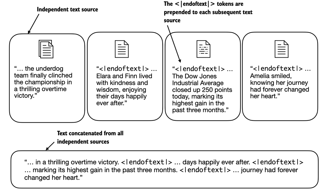
Figure 2.10 When working with multiple independent text source, we add <|endoftext|> tokens between these texts. These <|endoftext|> tokens act as markers, signaling the start or end of a particular segment, allowing for more effective processing and understanding by the LLM.
Let's now modify the vocabulary to include these two special tokens, <unk> and <|endoftext|>, by adding these to the list of all unique words that we created in the previous section:
all_words.extend(["<|endoftext|>", "<|unk|>"]) vocab = {token:integer for integer,token in enumerate(all_tokens)} print(len(vocab.items())) Based on the output of the print statement above, the new vocabulary size is 1161 (the vocabulary size in the previous section was 1159).
As an additional quick check, let's print the last 5 entries of the updated vocabulary:
for i, item in enumerate(list(vocab.items())[-5:]): print(item)
The code above prints the following:
('younger', 1156) ('your', 1157) ('yourself', 1158) ('<|endoftext|>', 1159) ('<|unk|>', 1160) Based on the code output above, we can confirm that the two new special tokens were indeed successfully incorporated into the vocabulary. Next, we adjust the tokenizer from code listing 2.3 accordingly, as shown in listing 2.4:
Listing 2.4 A simple text tokenizer that handles unknown words
class SimpleTokenizerV2: def __init__(self, vocab): self.str_to_int = vocab self.int_to_str = { i:s for s,i in vocab.items()} def encode(self, text): preprocessed = re.split(r'([,.?_!"()\']|--|\s)', text) preprocessed = [item.strip() for item in preprocessed if item.strip()] preprocessed = [item if item in self.str_to_int #A else "<|unk|>" for item in preprocessed] ids = [self.str_to_int[s] for s in preprocessed] return ids def decode(self, ids): text = " ".join([self.int_to_str[i] for i in ids]) text = re.sub(r'\s+([,.?!"()\'])', r'\1', text) #B return text Compared to the SimpleTokenizerV1 we implemented in code listing 2.3 in the previous section, the new SimpleTokenizerV2 replaces unknown words by <|unk|> tokens.
Let's now try this new tokenizer out in practice. For this, we will use a simple text sample that we concatenate from two independent and unrelated sentences:
text1 = "Hello, do you like tea?" text2 = "In the sunlit terraces of the palace." text = " <|endoftext|> ".join((text1, text2)) print(text)
The output is as follows:
'Hello, do you like tea? <|endoftext|> In the sunlit terraces of the palace.'
Next, let's tokenize the sample text using the SimpleTokenizerV2:
tokenizer = SimpleTokenizerV2(vocab) print(tokenizer.encode(text))
This prints the following token IDs:
[1160, 5, 362, 1155, 642, 1000, 10, 1159, 57, 1013, 981, 1009, 738, 1013, 1160, 7]
Above, we can see that the list of token IDs contains 1159 for the <|endoftext|> separator token as well as two 160 tokens, which are used for unknown words.
Let's de-tokenize the text for a quick sanity check:
print(tokenizer.decode(tokenizer.encode(text)))
The output is as follows:
'<|unk|>, do you like tea? <|endoftext|> In the sunlit terraces of the <|unk|>.'
Based on comparing the de-tokenized text above with the original input text, we know that the training dataset, Edith Wharton's short story The Verdict, did not contain the words "Hello" and "palace."
So far, we have discussed tokenization as an essential step in processing text as input to LLMs. Depending on the LLM, some researchers also consider additional special tokens such as the following:
- [BOS] (beginning of sequence): This token marks the start of a text. It signifies to the LLM where a piece of content begins.
- [EOS] (end of sequence): This token is positioned at the end of a text, and is especially useful when concatenating multiple unrelated texts, similar to <|endoftext|>. For instance, when combining two different Wikipedia articles or books, the [EOS] token indicates where one article ends and the next one begins.
- [PAD] (padding): When training LLMs with batch sizes larger than one, the batch might contain texts of varying lengths. To ensure all texts have the same length, the shorter texts are extended or "padded" using the [PAD] token, up to the length of the longest text in the batch.
Note that the tokenizer used for GPT models does not need any of these tokens mentioned above but only uses an <|endoftext|> token for simplicity. The <|endoftext|> is analogous to the [EOS] token mentioned above. Also, <|endoftext|> is used for padding as well. However, as we'll explore in subsequent chapters when training on batched inputs, we typically use a mask, meaning we don't attend to padded tokens. Thus, the specific token chosen for padding becomes inconsequential.
Moreover, the tokenizer used for GPT models also doesn't use an <|unk|> token for out-of-vocabulary words. Instead, GPT models use a byte pair encoding tokenizer, which breaks down words into subword units, which we will discuss in the next section.
2.5 Byte pair encoding
We implemented a simple tokenization scheme in the previous sections for illustration purposes. This section covers a more sophisticated tokenization scheme based on a concept called byte pair encoding (BPE). The BPE tokenizer covered in this section was used to train LLMs such as GPT-2, GPT-3, and ChatGPT.
Since implementing BPE can be relatively complicated, we will use an existing Python open-source library called tiktoken (https://github.com/openai/tiktoken), which implements the BPE algorithm very efficiently based on source code in Rust. Similar to other Python libraries, we can install the tiktoken library via Python's pip installer from the terminal:
pip install tiktoken
The code in this chapter is based on tiktoken 0.5.1. You can use the following code to check the version you currently have installed:
import importlib import tiktoken print("tiktoken version:", importlib.metadata.version("tiktoken")) Once installed, we can instantiate the BPE tokenizer from tiktoken as follows:
tokenizer = tiktoken.get_encoding("gpt2") The usage of this tokenizer is similar to SimpleTokenizerV2 we implemented previously via an encode method:
text = "Hello, do you like tea? <|endoftext|> In the sunlit terraces of someunknownPlace." integers = tokenizer.encode(text, allowed_special={"<|endoftext|>"}) print(integers) The code above prints the following token IDs:
[15496, 11, 466, 345, 588, 8887, 30, 220, 50256, 554, 262, 4252, 18250, 8812, 2114, 286, 617, 34680, 27271, 13]
We can then convert the token IDs back into text using the decode method, similar to our SimpleTokenizerV2 earlier:
strings = tokenizer.decode(integers) print(strings)
The above code prints the following:
'Hello, do you like tea? <|endoftext|> In the sunlit terraces of someunknownPlace.'
We can make two noteworthy observations based on the token IDs and decoded text above. First, the <|endoftext|> token is assigned a relatively large token ID, namely, 50256. In fact, the BPE tokenizer that was used to train models such as GPT-2, GPT-3, and ChatGPT has a total vocabulary size of 50,257, with <|endoftext|> being assigned the largest token ID.
Second, the BPE tokenizer above encodes and decodes unknown words, such as "someunknownPlace" correctly. The BPE tokenizer can handle any unknown word. How does it achieve this without using <|unk|> tokens?
The algorithm underlying BPE breaks down words that aren't in its predefined vocabulary into smaller subword units or even individual characters, enabling it to handle out-of-vocabulary words. So, thanks to the BPE algorithm, if the tokenizer encounters an unfamiliar word during tokenization, it can represent it as a sequence of subword tokens or characters, as illustrated in figure 2.11.
Figure 2.11 BPE tokenizers break down unknown words into subwords and individual characters. This way, a BPE tokenizer can parse any word and doesn't need to replace unknown words with special tokens, such as <|unk|>.
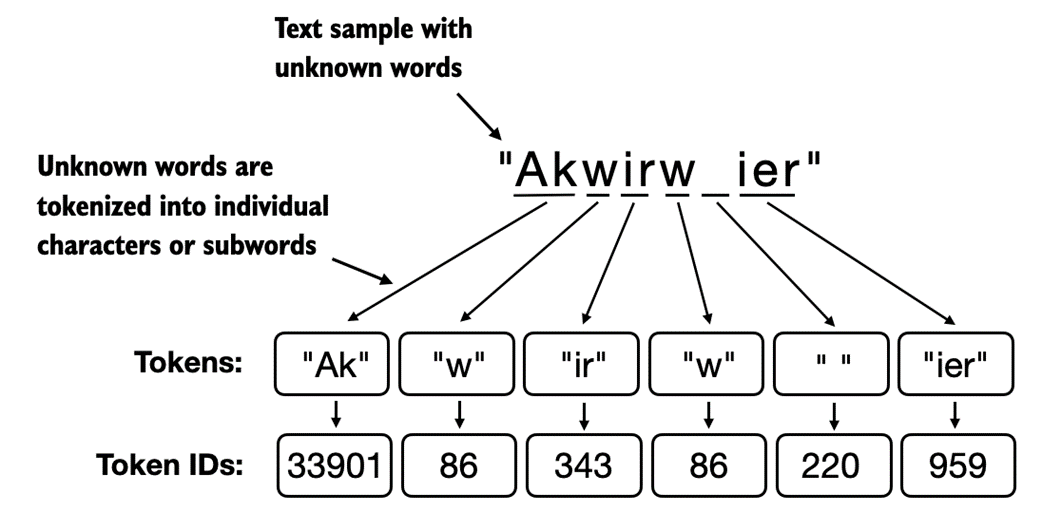
As illustrated in figure 2.11, the ability to break down unknown words into individual characters ensures that the tokenizer, and consequently the LLM that is trained with it, can process any text, even if it contains words that were not present in its training data.
Exercise 2.1 Byte pair encoding of unknown words
Try the BPE tokenizer from the tiktoken library on the unknown words "Akwirw ier" and print the individual token IDs. Then, call the decode function on each of the resulting integers in this list to reproduce the mapping shown in figure 2.1. Lastly, call the decode method on the token IDs to check whether it can reconstruct the original input, "Akwirw ier".
A detailed discussion and implementation of BPE is out of the scope of this book, but in short, it builds its vocabulary by iteratively merging frequent characters into subwords and frequent subwords into words. For example, BPE starts with adding all individual single characters to its vocabulary ("a", "b", ...). In the next stage, it merges character combinations that frequently occur together into subwords. For example, "d" and "e" may be merged into the subword "de," which is common in many English words like "define", "depend", "made", and "hidden". The merges are determined by a frequency cutoff.
2.6 Data sampling with a sliding window
The previous section covered the tokenization steps and conversion from string tokens into integer token IDs in great detail. The next step before we can finally create the embeddings for the LLM is to generate the input-target pairs required for training an LLM.
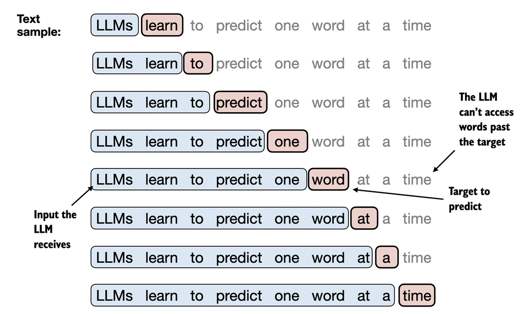
What do these input-target pairs look like? As we learned in chapter 1, LLMs are pretrained by predicting the next word in a text, as depicted in figure 2.12.
Figure 2.12 Given a text sample, extract input blocks as subsamples that serve as input to the LLM, and the LLM's prediction task during training is to predict the next word that follows the input block. During training, we mask out all words that are past the target. Note that the text shown in this figure would undergo tokenization before the LLM can process it; however, this figure omits the tokenization step for clarity.
In this section we implement a data loader that fetches the input-target pairs depicted in figure 2.12 from the training dataset using a sliding window approach.
To get started, we will first tokenize the whole The Verdict short story we worked with earlier using the BPE tokenizer introduced in the previous section:
with open("the-verdict.txt", "r", encoding="utf-8") as f: raw_text = f.read() enc_text = tokenizer.encode(raw_text) print(len(enc_text)) Executing the code above will return 5145, the total number of tokens in the training set, after applying the BPE tokenizer.
Next, we remove the first 50 tokens from the dataset for demonstration purposesas it results in a slightly more interesting text passage in the next steps:
enc_sample = enc_text[50:]
One of the easiest and most intuitive ways to create the input-target pairs for the next-word prediction task is to create two variables, x and y, where x contains the input tokens and y contains the targets, which are the inputs shifted by 1:
context_size = 4 #A x = enc_sample[:context_size] y = enc_sample[1:context_size+1] print(f"x: {x}") print(f"y: {y}") Running the above code prints the following output:
x: [290, 4920, 2241, 287] y: [4920, 2241, 287, 257]
Processing the inputs along with the targets, which are the inputs shifted by one position, we can then create the next-word prediction tasks depicted earlier in figure 2.12, as follows:
for i in range(1, context_size+1): context = enc_sample[:i] desired = enc_sample[i] print(context, "---->", desired)
The code above prints the following:
[290] ----> 4920 [290, 4920] ----> 2241 [290, 4920, 2241] ----> 287 [290, 4920, 2241, 287] ----> 257
Everything left of the arrow (---->) refers to the input an LLM would receive, and the token ID on the right side of the arrow represents the target token ID that the LLM is supposed to predict.
For illustration purposes, let's repeat the previous code but convert the token IDs into text:
for i in range(1, context_size+1): context = enc_sample[:i] desired = enc_sample[i] print(tokenizer.decode(context), "---->", tokenizer.decode([desired]))
The following outputs show how the input and outputs look in text format:
and ----> established and established ----> himself and established himself ----> in and established himself in ----> a
We've now created the input-target pairs that we can turn into use for the LLM training in upcoming chapters.
There's only one more task before we can turn the tokens into embeddings, as we mentioned at the beginning of this chapter: implementing an efficient data loader that iterates over the input dataset and returns the inputs and targets as PyTorch tensors.
In particular, we are interested in returning two tensors: an input tensor containing the text that the LLM sees and a target tensor that includes the targets for the LLM to predict, as depicted in figure 2.13.
Figure 2.13 To implement efficient data loaders, we collect the inputs in a tensor, x, where each row represents one input context. A second tensor, y, contains the corresponding prediction targets (next words), which are created by shifting the input by one position.
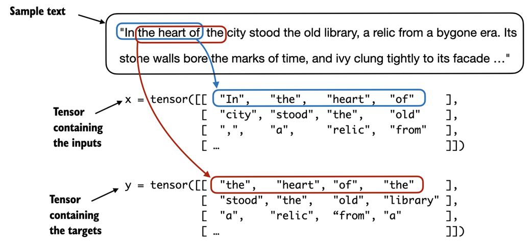
While figure 2.13 shows the tokens in string format for illustration purposes, the code implementation will operate on token IDs directly since the encode method of the BPE tokenizer performs both tokenization and conversion into token IDs as a single step.
For the efficient data loader implementation, we will use PyTorch's built-in Dataset and DataLoader classes. For additional information and guidance on installing PyTorch, please see section A.1.3, Installing PyTorch, in Appendix A.
The code for the dataset class is shown in code listing 2.5:
Listing 2.5 A dataset for batched inputs and targets
import torch from torch.utils.data import Dataset, DataLoader class GPTDatasetV1(Dataset): def __init__(self, txt, tokenizer, max_length, stride): self.tokenizer = tokenizer self.input_ids = [] self.target_ids = [] token_ids = tokenizer.encode(txt) #A for i in range(0, len(token_ids) - max_length, stride): #B input_chunk = token_ids[i:i + max_length] target_chunk = token_ids[i + 1: i + max_length + 1] self.input_ids.append(torch.tensor(input_chunk)) self.target_ids.append(torch.tensor(target_chunk)) def __len__(self): #C return len(self.input_ids) def __getitem__(self, idx): #D return self.input_ids[idx], self.target_ids[idx]
The GPTDatasetV1 class in listing 2.5 is based on the PyTorch Dataset class and defines how individual rows are fetched from the dataset, where each row consists of a number of token IDs (based on a max_length) assigned to an input_chunk tensor. The target_chunk tensor contains the corresponding targets. I recommend reading on to see how the data returned from this dataset looks like when we combine the dataset with a PyTorch DataLoader -- this will bring additional intuition and clarity.
If you are new to the structure of PyTorch Dataset classes, such as shown in listing 2.5, please read section A.6, Setting up efficient data loaders, in Appendix A, which explains the general structure and usage of PyTorch Dataset and DataLoader classes.
The following code will use the GPTDatasetV1 to load the inputs in batches via a PyTorch DataLoader:
Listing 2.6 A data loader to generate batches with input-with pairs
def create_dataloader(txt, batch_size=4, max_length=256, stride=128): tokenizer = tiktoken.get_encoding("gpt2") #A dataset = GPTDatasetV1(txt, tokenizer, max_length, stride) #B dataloader = DataLoader(dataset, batch_size=batch_size) #C return dataloader Let's test the dataloader with a batch size of 1 for an LLM with a context size of 4 to develop an intuition of how the GPTDatasetV1 class from listing 2.5 and the create_dataloader function from listing 2.6 work together:
with open("the-verdict.txt", "r", encoding="utf-8") as f: raw_text = f.read() dataloader = create_dataloader(raw_text, batch_size=1, max_length=4, stride=1) data_iter = iter(dataloader) #A first_batch = next(data_iter) print(first_batch) Executing the preceding code prints the following:
[tensor([[ 40, 367, 2885, 1464]]), tensor([[ 367, 2885, 1464, 1807]])]
The first_batch variable contains two tensors: the first tensor stores the input token IDs, and the second tensor stores the target token IDs. Since the max_length is set to 4, each of the two tensors contains 4 token IDs. Note that an input size of 4 is relatively small and only chosen for illustration purposes. It is common to train LLMs with input sizes of at least 256.
To illustrate the meaning of stride=1, let's fetch another batch from this dataset:
second_batch = next(data_iter) print(second_batch)
The second batch has the following contents:
[tensor([[ 367, 2885, 1464, 1807]]), tensor([[2885, 1464, 1807, 3619]])]
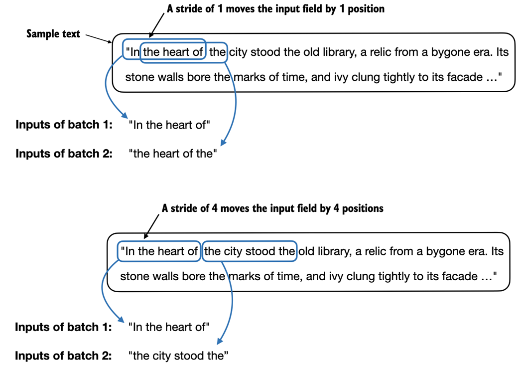
If we compare the first with the second batch, we can see that the second batch's token IDs are shifted by one position compared to the first batch (for example, the second ID in the first batch's input is 367, which is the first ID of the second batch's input). The stride setting dictates the number of positions the inputs shift across batches, emulating a sliding window approach, as demonstrated in Figure 2.14.
Figure 2.14 When creating multiple batches from the input dataset, we slide an input window across the text. If the stride is set to 1, we shift the input window by 1 position when creating the next batch. If we set the stride equal to the input window size, we can prevent overlaps between the batches.
Exercise 2.2 Data loaders with different strides and context sizes
To develop more intuition for how the data loader works, try to run it with different settings such as max_length=2 and stride=2 and max_length=8 and stride=2.
Batch sizes of 1, such as we have sampled from the data loader so far, are useful for illustration purposes. If you have previous experience with deep learning, you may know that small batch sizes require less memory during training but lead to more noisy model updates. Just like in regular deep learning, the batch size is a trade-off and hyperparameter to experiment with when training LLMs.
Before we move on to the two final sections of this chapter that are focused on creating the embedding vectors from the token IDs, let's have a brief look at how we can use the data loader to sample with a batch size greater than 1:
dataloader = create_dataloader(raw_text, batch_size=8, max_length=4, stride=5) data_iter = iter(dataloader) inputs, targets = next(data_iter) print("Inputs:\n", inputs) print("\nTargets:\n", targets) This prints the following:
Inputs: tensor([[ 40, 367, 2885, 1464], [ 3619, 402, 271, 10899], [ 257, 7026, 15632, 438], [ 257, 922, 5891, 1576], [ 568, 340, 373, 645], [ 5975, 284, 502, 284], [ 326, 11, 287, 262], [ 286, 465, 13476, 11]]) Targets: tensor([[ 367, 2885, 1464, 1807], [ 402, 271, 10899, 2138], [ 7026, 15632, 438, 2016], [ 922, 5891, 1576, 438], [ 340, 373, 645, 1049], [ 284, 502, 284, 3285], [ 11, 287, 262, 6001], [ 465, 13476, 11, 339]])
Note that we increase the stride to 5, which is the max length + 1. This is to utilize the data set fully (we don't skip a single word) but also avoid any overlap between the batches, since more overlap could lead to increased overfitting. For instance, if we set the stride equal to the max length, the target ID for the last input token ID in each row would become the first input token ID in the next row.
In the final two sections of this chapter, we will implement embedding layers that convert the token IDs into continuous vector representations, which serve as input data format for LLMs.
2.7 Creating token embeddings
The last step for preparing the input text for LLM training is to convert the token IDs into embedding vectors, as illustrated in figure 2.15, which will be the focus of these two last remaining sections of this chapter.
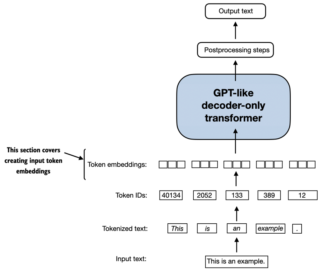
Figure 2.15 Preparing the input text for an LLM involves tokenizing text, converting text tokens to token IDs, and converting token IDs into vector embedding vectors. In this section, we consider the token IDs created in previous sections to create the token embedding vectors.
A continuous vector representation, or embedding, is necessary since GPT-like LLMs are deep neural networks trained with the backpropagation algorithm. If you are unfamiliar with how neural networks are trained with backpropagation, please read section A.4, Automatic differentiation made easy, in Appendix A.
Let's illustrate how the token ID to embedding vector conversion works with a hands-on example. Suppose we have the following three input tokens with IDs 5, 1, 3, and 2:
input_ids = torch.tensor([5, 1, 3, 2])
For the sake of simplicity and illustration purposes, suppose we have a small vocabulary of only 6 words (instead of the 50,257 words in the BPE tokenizer vocabulary), and we want to create embeddings of size 3 (in GPT-3, the embedding size is 12,288 dimensions):
vocab_size = 6 output_dim = 3
Using the vocab_size and output_dim, we can instantiate an embedding layer in PyTorch, setting the random seed to 123 for reproducibility purposes:
torch.manual_seed(123) embedding_layer = torch.nn.Embedding(vocab_size, output_dim) print(embedding_layer.weight)
The print statement in the preceding code example prints the embedding layer's underlying weight matrix:
Parameter containing: tensor([[ 0.3374, -0.1778, -0.1690], [ 0.9178, 1.5810, 1.3010], [ 1.2753, -0.2010, -0.1606], [-0.4015, 0.9666, -1.1481], [-1.1589, 0.3255, -0.6315], [-2.8400, -0.7849, -1.4096]], requires_grad=True)
We can see that the weight matrix of the embedding layer contains small, random values. These values are optimized during LLM training as part of the LLM optimization itself, as we will see in upcoming chapters. Moreover, we can see that the weight matrix has six rows and three columns. There is one row for each of the six possible tokens in the vocabulary. And there is one column for each of the three embedding dimensions.
After we instantiated the embedding layer, let's now apply it to a token ID to obtain the embedding vector:
print(embedding_layer(torch.tensor([3])))
The returned embedding vector is as follows:
tensor([[-0.4015, 0.9666, -1.1481]], grad_fn=<EmbeddingBackward0>)
If we compare the embedding vector for token ID 3 to the previous embedding matrix, we see that it is identical to the 4th row (Python starts with a zero index, so it's the row corresponding to index 3). In other words, the embedding layer is essentially a look-up operation that retrieves rows from the embedding layer's weight matrix via a token ID.
Embedding layers versus matrix multiplication
For those who are familiar with one-hot encoding, the embedding layer approach above is essentially just a more efficient way of implementing one-hot encoding followed by matrix multiplication in a fully connected layer, which is illustrated in the supplementary code on GitHub at https://github.com/rasbt/LLMs-from-scratch/tree/main/ch02/03_bonus_embedding-vs-matmul. Because the embedding layer is just a more efficient implementation equivalent to the one-hot encoding and matrix-multiplication approach, it can be seen as a neural network layer that can be optimized via backpropagation.
Previously, we have seen how to convert a single token ID into a three-dimensional embedding vector. Let's now apply that to all four input IDs we defined earlier (torch.tensor([5, 1, 3, 2])):
print(embedding_layer(input_ids))
The print output reveals that this results in a 4x3 matrix:
tensor([[-2.8400, -0.7849, -1.4096], [ 0.9178, 1.5810, 1.3010], [-0.4015, 0.9666, -1.1481], [ 1.2753, -0.2010, -0.1606]], grad_fn=<EmbeddingBackward0>)
Each row in this output matrix is obtained via a lookup operation from the embedding weight matrix, as illustrated in figure 2.16.
Figure 2.16 Embedding layers perform a look-up operation, retrieving the embedding vector corresponding to the token ID from the embedding layer's weight matrix. For instance, the embedding vector of the token ID 5 is the sixth row of the embedding layer weight matrix (it is the sixth instead of the fifth row because Python starts counting at 0).
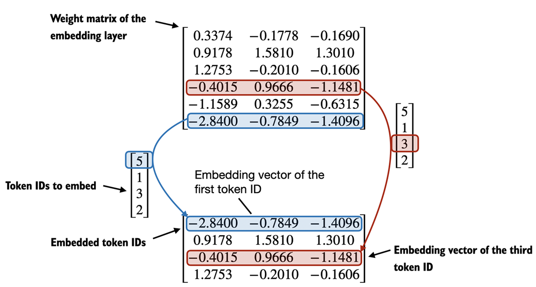
This section covered how we create embedding vectors from token IDs. The next and final section of this chapter will add a small modification to these embedding vectors to encode positional information about a token within a text.
2.8 Encoding word positions
In the previous section, we converted the token IDs into a continuous vector representation, the so-called token embeddings. In principle, this is a suitable input for an LLM. However, a minor shortcoming of LLMs is that their self-attention mechanism, which will be covered in detail in chapter 3, doesn't have a notion of position or order for the tokens within a sequence.
The way the previously introduced embedding layer works is that the same token ID always gets mapped to the same vector representation, regardless of where the token ID is positioned in the input sequence, as illustrated in figure 2.17.
Figure 2.17 The embedding layer converts a token ID into the same vector representation regardless of where it is located in the input sequence. For example, the token ID 5, whether it's in the first or third position in the token ID input vector, will result in the same embedding vector.
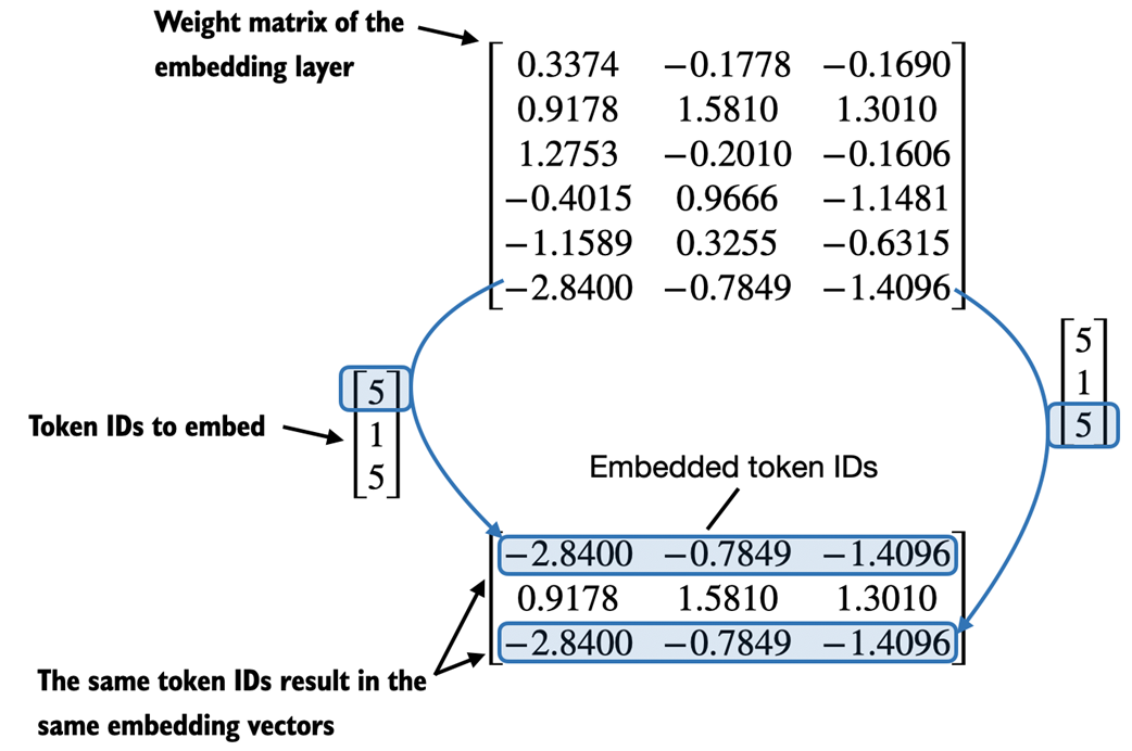
In principle, the deterministic, position-independent embedding of the token ID is good for reproducibility purposes. However, since the self-attention mechanism of LLMs itself is also position-agnostic, it is helpful to inject additional position information into the LLM.
To achieve this, there are two broad categories of position-aware embeddings: relative positional embeddings and absolute positional embeddings.
Absolute positional embeddings are directly associated with specific positions in a sequence. For each position in the input sequence, a unique embedding is added to the token's embedding to convey its exact location. For instance, the first token will have a specific positional embedding, the second token another distinct embedding, and so on, as illustrated in figure 2.18.
Figure 2.18 Positional embeddings are added to the token embedding vector to create the input embeddings for an LLM. The positional vectors have the same dimension as the original token embeddings. The token embeddings are shown with value 1 for simplicity.
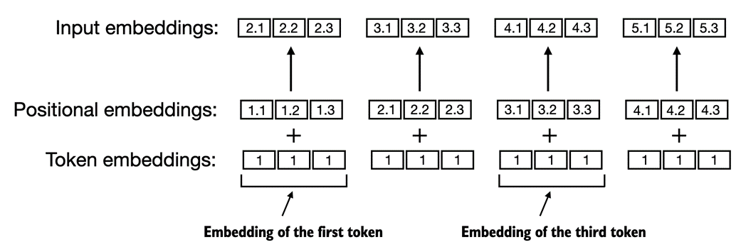
Instead of focusing on the absolute position of a token, the emphasis of relative positional embeddings is on the relative position or distance between tokens. This means the model learns the relationships in terms of "how far apart" rather than "at which exact position." The advantage here is that the model can generalize better to sequences of varying lengths, even if it hasn't seen such lengths during training.
Both types of positional embeddings aim to augment the capacity of LLMs to understand the order and relationships between tokens, ensuring more accurate and context-aware predictions. The choice between them often depends on the specific application and the nature of the data being processed.
OpenAI's GPT models use absolute positional embeddings that are optimized during the training process rather than being fixed or predefined like the positional encodings in the original Transformer model. This optimization process is part of the model training itself, which we will implement later in this book. For now, let's create the initial positional embeddings to create the LLM inputs for the upcoming chapters.
Previously, we focused on very small embedding sizes in this chapter for illustration purposes. We now consider more realistic and useful embedding sizes and encode the input tokens into a 256-dimensional vector representation. This is smaller than what the original GPT-3 model used (in GPT-3, the embedding size is 12,288 dimensions) but still reasonable for experimentation. Furthermore, we assume that the token IDs were created by the BPE tokenizer that we implemented earlier, which has a vocabulary size of 50,257:
output_dim = 256 vocab_size = 50257 token_embedding_layer = torch.nn.Embedding(vocab_size, output_dim)
Using the token_embedding_layer above, if we sample data from the data loader, we embed each token in each batch into a 256-dimensional vector. If we have a batch size of 8 with four tokens each, the result will be an 8 x 4 x 256 tensor.
Let's instantiate the data loader from section 2.6, Data sampling with a sliding window, first:
max_length = 4 dataloader = create_dataloader( raw_text, batch_size=8, max_length=max_length, stride=5) data_iter = iter(dataloader) inputs, targets = next(data_iter) print("Token IDs:\n", inputs) print("\nInputs shape:\n", inputs.shape) The preceding code prints the following output:
Token IDs: tensor([[ 40, 367, 2885, 1464], [ 3619, 402, 271, 10899], [ 257, 7026, 15632, 438], [ 257, 922, 5891, 1576], [ 568, 340, 373, 645], [ 5975, 284, 502, 284], [ 326, 11, 287, 262], [ 286, 465, 13476, 11]]) Inputs shape: torch.Size([8, 4])
As we can see, the token ID tensor is 8x4-dimensional, meaning that the data batch consists of 8 text samples with 4 tokens each.
Let's now use the embedding layer to embed these token IDs into 256-dimensional vectors:
token_embeddings = token_embedding_layer(inputs) print(token_embeddings.shape)
The preceding print function call returns the following:
torch.Size([8, 4, 256])
As we can tell based on the 8x4x256-dimensional tensor output, each token ID is now embedded as a 256-dimensional vector.
For a GPT model's absolute embedding approach, we just need to create another embedding layer that has the same dimension as the token_embedding_layer:
block_size = max_length pos_embedding_layer = torch.nn.Embedding(block_size, output_dim) pos_embeddings = pos_embedding_layer(torch.arange(block_size)) print(pos_embeddings.shape)
As shown in the preceding code example, the input to the pos_embeddings is usually a placeholder vector torch.arange(block_size), which contains a sequence of numbers 1, 2, ..., up to the maximum input length. The block_size is a variable that represents the supported input size of the LLM. Here, we choose it similar to the maximum length of the input text. In practice, input text can be longer than the supported block size, in which case we have to truncate the text. The text can also be shorter than the block size, in which case we fill in the remaining input with placeholder tokens to match the block size, as we will see in chapter 3.
The output of the print statement is as follows:
torch.Size([4, 256])
As we can see, the positional embedding tensor consists of four 256-dimensional vectors. We can now add these directly to the token embeddings, where PyTorch will add the 4x256-dimensional pos_embeddings tensor to each 4x256-dimensional token embedding tensor in each of the 8 batches:
input_embeddings = token_embeddings + pos_embeddings print(input_embeddings.shape)
The print output is as follows:
torch.Size([8, 4, 256])
The input_embeddings we created, as summarized in figure 2.19, are the embedded input examples that can now be processed by the main LLM modules, which we will begin implementing in chapter 3
Figure 2.19 As part of the input processing pipeline, input text is first broken up into individual tokens. These tokens are then converted into token IDs using a vocabulary. The token IDs are converted into embedding vectors to which positional embeddings of a similar size are added, resulting in input embeddings that are used as input for the main LLM layers.
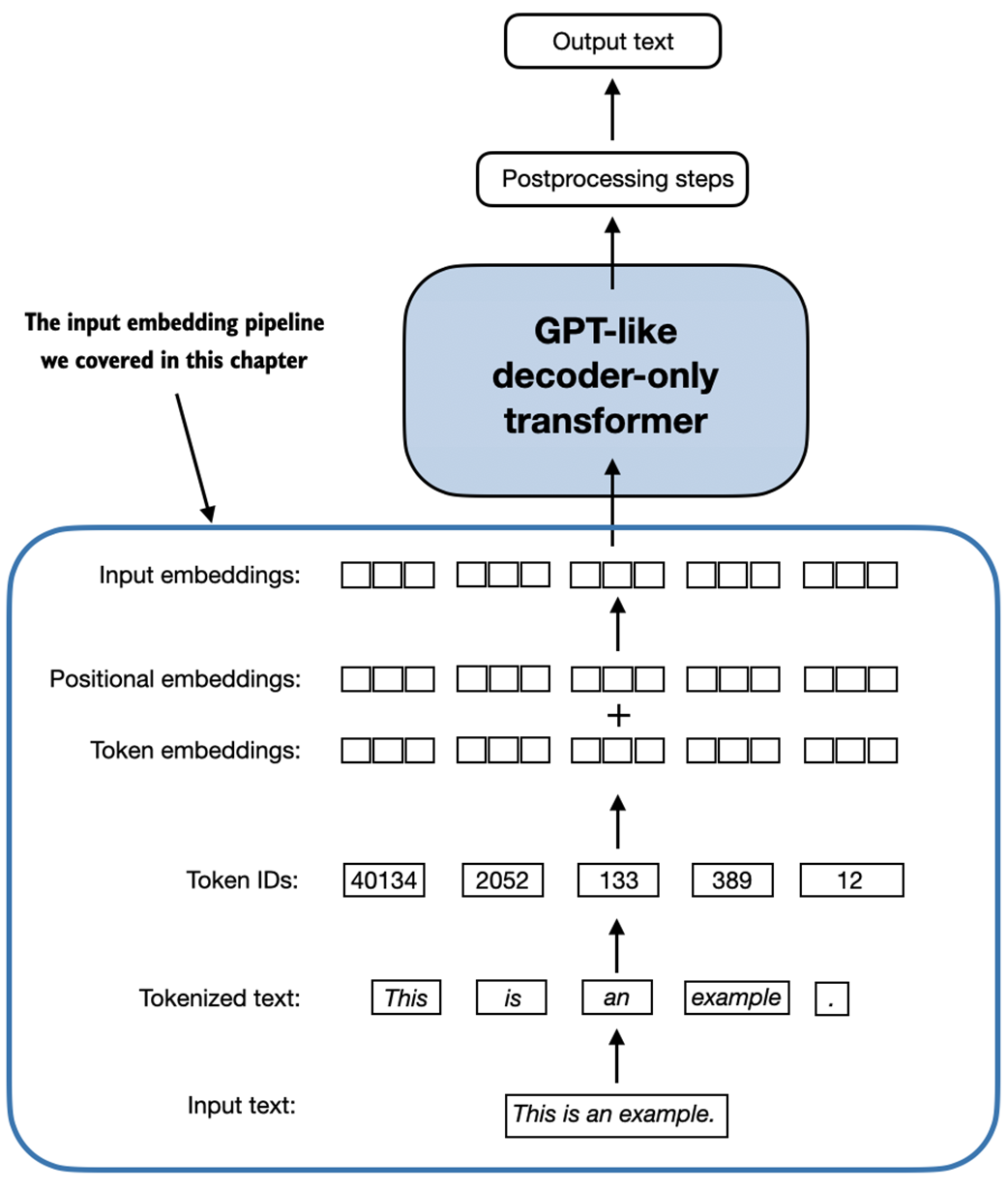
2.9 Summary
- LLMs require textual data to be converted into numerical vectors, known as embeddings since they can't process raw text. Embeddings transform discrete data (like words or images) into continuous vector spaces, making them compatible with neural network operations.
- As the first step, raw text is broken into tokens, which can be words or characters. Then, the tokens are converted into integer representations, termed token IDs.
- Special tokens, such as <|unk|> and <|endoftext|>, can be added to enhance the model's understanding and handle various contexts, such as unknown words or marking the boundary between unrelated texts.
- The byte pair encoding (BPE) tokenizer used for LLMs like GPT-2 and GPT-3 can efficiently handle unknown words by breaking them down into subword units or individual characters.
- We use a sliding window approach on tokenized data to generate input-target pairs for LLM training.
- Embedding layers in PyTorch function as a lookup operation, retrieving vectors corresponding to token IDs. The resulting embedding vectors provide continuous representations of tokens, which is crucial for training deep learning models like LLMs.
- While token embeddings provide consistent vector representations for each token, they lack a sense of the token's position in a sequence. To rectify this, two main types of positional embeddings exist: absolute and relative. OpenAI's GPT models utilize absolute positional embeddings that are added to the token embedding vectors and are optimized during the model training.
2.10 References and further reading
Readers who are interested in discussion and comparison of embedding spaces with latent spaces and the general notion of vector representations can find more information in the first chapter of my book Machine Learning Q and AI:
- Machine Learning Q and AI (2023) by Sebastian Raschka, https://leanpub.com/machine-learning-q-and-ai
- The following paper provides more in-depth discussions of how how byte pair encoding is used as a tokenization method:
- Neural Machine Translation of Rare Words with Subword Units (2015) by Sennrich at al., https://arxiv.org/abs/1508.07909
- The code for the byte pair encoding tokenizer used to train GPT-2 was open-sourced by OpenAI:
- https://github.com/openai/gpt-2/blob/master/src/encoder.py
- OpenAI provides an interactive web UI to illustrate how the byte pair tokenizer in GPT models works:
- https://platform.openai.com/tokenizer
- Readers who are interested in studying alternative tokenization schemes that are used by some other popular LLMs can find more information in the SentencePiece and WordPiece papers:
- SentencePiece: A Simple and Language Independent Subword Tokenizer and Detokenizer for Neural Text Processing (2018) by Kudo and Richardson, https://aclanthology.org/D18-2012/
- Fast WordPiece Tokenization (2020) by Song et al., https://arxiv.org/abs/2012.15524
2.11 Exercise answers
The complete code examples for the exercises answers can be found in the supplementary GitHub repository at https://github.com/rasbt/LLMs-from-scratch
Exercise 2.1
You can obtain the individual token IDs by prompting the encoder with one string at a time:
print(tokenizer.encode("Ak")) print(tokenizer.encode("w")) # ... This prints:
[33901] [86] # ...
You can then use the following code to assemble the original string:
welcome
Thank you for purchasing the MEAP edition of Build a Large Language Model (From Scratch).
In this book, I invite you to embark on an educational journey with me to learn how to build Large Language Models (LLMs) from the ground up. Together, we'll delve deep into the LLM training pipeline, starting from data loading and culminating in finetuning LLMs on custom datasets.
For many years, I've been deeply immersed in the world of deep learning, coding LLMs, and have found great joy in explaining complex concepts thoroughly. This book has been a long-standing idea in my mind, and I'm thrilled to finally have the opportunity to write it and share it with you. Those of you familiar with my work, especially from my blog, have likely seen glimpses of my approach to coding from scratch. This method has resonated well with many readers, and I hope it will be equally effective for you.
I've designed the book to emphasize hands-on learning, primarily using PyTorch and without relying on pre-existing libraries. With this approach, coupled with numerous figures and illustrations, I aim to provide you with a thorough understanding of how LLMs work, their limitations, and customization methods. Moreover, we'll explore commonly used workflows and paradigms in pretraining and fine-tuning LLMs, offering insights into their development and customization.
The book is structured with detailed step-by-step introductions, ensuring no critical detail is overlooked. To gain the most from this book, you should have a background in Python programming. Prior experience in deep learning and a foundational understanding of PyTorch, or familiarity with other deep learning frameworks like TensorFlow, will be beneficial.
I warmly invite you to engage in the liveBook discussion forum for any questions, suggestions, or feedback you might have. Your contributions are immensely valuable and appreciated in enhancing this learning journey.
— Sebastian Raschka